Do the Data Meet the Assumption of Equal Variances? How Do You Know?

Introduction

Linear regression models observe several uses in real-life issues. For case, a multi-national corporation wanting to identify factors that can affect the sales of its production tin can run a linear regression to find out which factors are important. In econometrics, Ordinary Least Squares (OLS) method is widely used to approximate the parameter of a linear regression model. OLS estimators minimize the sum of the squared errors (a difference betwixt observed values and predicted values). While OLS is computationally feasible and can be easily used while doing any econometrics test, it is important to know the underlying assumptions of OLS regression. This is considering a lack of knowledge of OLS assumptions would result in its misuse and give incorrect results for the econometrics test completed. The importance of OLS assumptions cannot be overemphasized. The next department describes the assumptions of OLS regression.

Assumptions of OLS Regression

The necessary OLS assumptions, which are used to derive the OLS estimators in linear regression models, are discussed below.

OLS Supposition i: The linear regression model is "linear in parameters."

When the dependent variable (Y) is a linear function of contained variables (X's) and the error term, the regression is linear in parameters and not necessarily linear in X's. For example, consider the post-obit:

A1. The linear regression model is "linear in parameters."

A2. There is a random sampling of observations.

A3. The provisional mean should be zero.

A4. There is no multi-collinearity (or perfect collinearity).

A5. Spherical errors: At that place is homoscedasticity and no autocorrelation

A6: Optional Assumption: Error terms should be normally distributed.

a)\quad Y={ \beta }_{ 0 }+{ \beta }_{ i }{ Ten }_{ 1 }+{ \beta }_{ 2 }{ X }_{ two }+\varepsilon

b)\quad Y={ \beta }_{ 0 }+{ \beta }_{ 1 }{ Ten }_{ { 1 }^{ ii } }+{ \beta }_{ 2 }{ X }_{ 2 }+\varepsilon

c)\quad Y={ \beta }_{ 0 }+{ \beta }_{ { ane }^{ 2 } }{ 10 }_{ one }+{ \beta }_{ two }{ X }_{ 2 }+\varepsilon

In the above three examples, for a) and b) OLS assumption 1 is satisfied. For c) OLS assumption 1 is not satisfied because it is not linear in parameter { \beta }_{ 1 }.

OLS Supposition 2: In that location is a random sampling of observations

This assumption of OLS regression says that:

• The sample taken for the linear regression model must be drawn randomly from the population. For example, if you have to run a regression model to study the factors that impact the scores of students in the last exam, and then you must select students randomly from the university during your data collection procedure, rather than adopting a convenient sampling procedure.
• The number of observations taken in the sample for making the linear regression model should exist greater than the number of parameters to be estimated. This makes sense mathematically too. If a number of parameters to exist estimated (unknowns) are more than the number of observations, then estimation is not possible. If a number of parameters to be estimated (unknowns) equal the number of observations, then OLS is not required. You can only use algebra.
• The X's should be fixed (due east. contained variables should affect dependent variables). It should not exist the case that dependent variables impact contained variables. This is because, in regression models, the causal relationship is studied and there is not a correlation between the two variables. For example, if y'all run the regression with inflation equally your dependent variable and unemployment equally the contained variable, the OLS estimators are likely to be incorrect because with inflation and unemployment, nosotros wait correlation rather than a causal relationship.
• The error terms are random. This makes the dependent variable random.

OLS Assumption 3: The conditional hateful should be cipher.

The expected value of the mean of the error terms of OLS regression should exist zilch given the values of independent variables.

Mathematically, E\left( { \varepsilon }|{ X } \right) =0. This is sometimes just written as E\left( { \varepsilon } \right) =0.

In other words, the distribution of error terms has nil mean and doesn't depend on the contained variables X's. Thus, there must be no relationship betwixt the Ten'southward and the error term.

OLS Assumption 4: There is no multi-collinearity (or perfect collinearity).

In a simple linear regression model, there is merely i independent variable and hence, by default, this assumption will concur true. Still, in the case of multiple linear regression models, there are more than one independent variable. The OLS assumption of no multi-collinearity says that there should be no linear relationship between the contained variables. For example, suppose yous spend your 24 hours in a day on three things – sleeping, studying, or playing. Now, if you lot run a regression with dependent variable as exam score/performance and independent variables as fourth dimension spent sleeping, fourth dimension spent studying, and fourth dimension spent playing, and then this assumption will not hold.

This is because at that place is perfect collinearity between the three independent variables.

Time spent sleeping = 24 – Time spent studying – Time spent playing.

In such a situation, it is amend to drop ane of the iii independent variables from the linear regression model. If the relationship (correlation) betwixt contained variables is strong (simply not exactly perfect), information technology still causes issues in OLS estimators. Hence, this OLS assumption says that you should select independent variables that are not correlated with each other.

An important implication of this supposition of OLS regression is that there should be sufficient variation in the X's. More than the variability in X'due south, better are the OLS estimates in determining the impact of X's on Y.

OLS Supposition 5: Spherical errors: At that place is homoscedasticity and no autocorrelation.

According to this OLS assumption, the fault terms in the regression should all accept the same variance.

Mathematically, Var\left( { \varepsilon }|{ 10 } \right) ={ \sigma }^{ ii }.

If this variance is not abiding (i.e. dependent on X'south), and then the linear regression model has heteroscedastic errors and likely to requite incorrect estimates.

This OLS assumption of no autocorrelation says that the error terms of different observations should non be correlated with each other.

Mathematically, Cov\left( { { \varepsilon }_{ i }{ \varepsilon }_{ j } }|{ X } \right) =0\enspace for\enspace i\neq j

For example, when we have fourth dimension series data (east.g. yearly information of unemployment), so the regression is probable to suffer from autocorrelation considering unemployment next twelvemonth will certainly be dependent on unemployment this year. Hence, error terms in unlike observations will surely be correlated with each other.

In simple terms, this OLS assumption means that the fault terms should be IID (Independent and Identically Distributed).

Paradigm Source: Laerd Statistics

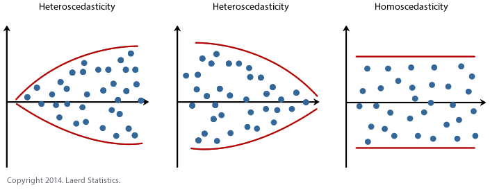
The to a higher place diagram shows the difference between Homoscedasticity and Heteroscedasticity. The variance of errors is constant in case of homoscedasticity while it's not the case if errors are heteroscedastic.

OLS Assumption 6: Fault terms should be normally distributed.

This assumption states that the errors are normally distributed, conditional upon the independent variables. This OLS supposition is not required for the validity of OLS method; all the same, it becomes of import when one needs to define some additional finite-sample properties. Note that merely the mistake terms need to exist usually distributed. The dependent variable Y need not be normally distributed.

The Use of OLS Assumptions

OLS assumptions are extremely important. If the OLS assumptions ane to five concord, and then co-ordinate to Gauss-Markov Theorem, OLS calculator is Best Linear Unbiased Reckoner (BLUE). These are desirable properties of OLS estimators and require split up give-and-take in detail. Withal, below the focus is on the importance of OLS assumptions past discussing what happens when they neglect and how can you look out for potential errors when assumptions are not outlined.

1. The Assumption of Linearity (OLS Assumption 1) – If you fit a linear model to a data that is not-linearly related, the model will be wrong and hence unreliable. When yous utilise the model for extrapolation, y'all are likely to get erroneous results. Hence, you should always plot a graph of observed predicted values. If this graph is symmetrically distributed forth the 45-caste line, so you can be sure that the linearity supposition holds. If linearity assumptions don't agree, and so you lot need to modify the functional grade of the regression, which can be done by taking non-linear transformations of contained variables (i.e. you can have log { X } instead of X equally your independent variable) and and then check for linearity.
2. The Supposition of Homoscedasticity (OLS Assumption 5) – If errors are heteroscedastic (i.e. OLS assumption is violated), then it volition be difficult to trust the standard errors of the OLS estimates. Hence, the confidence intervals will be either too narrow or besides wide. Likewise, violation of this supposition has a trend to give also much weight on some portion (subsection) of the data. Hence, it is important to set this if error variances are not constant. Y'all tin easily cheque if error variances are constant or non. Examine the plot of residuals predicted values or residuals vs. time (for time series models). Typically, if the data set is large, then errors are more or less homoscedastic. If your data set is pocket-sized, check for this assumption.
3. The Assumption of Independence/No Autocorrelation (OLS Assumption 5) – Every bit discussed previously, this assumption is most likely to be violated in fourth dimension series regression models and, hence, intuition says that there is no need to investigate it. However, you can all the same cheque for autocorrelation by viewing the residual time series plot. If autocorrelation is present in the model, you can try taking lags of independent variables to correct for the trend component. If you do not correct for autocorrelation, then OLS estimates won't be Blueish, and they won't exist reliable enough.
4. The Assumption of Normality of Errors (OLS Assumption 6) – If error terms are not normal, and so the standard errors of OLS estimates won't be reliable, which means the confidence intervals would exist too wide or narrow. Likewise, OLS estimators won't have the desirable Bluish belongings. A normal probability plot or a normal quantile plot tin exist used to bank check if the error terms are unremarkably distributed or non. A bow-shaped deviated design in these plots reveals that the errors are not normally distributed. Sometimes errors are non normal because the linearity assumption is non property. And then, it is worthwhile to check for linearity assumption again if this assumption fails.
5. Assumption of No Multicollinearity (OLS assumption four) – Yous can check for multicollinearity by making a correlation matrix (though in that location are other complex means of checking them like Variance Inflation Cistron, etc.). Almost a sure indication of the presence of multi-collinearity is when you get contrary (unexpected) signs for your regression coefficients (due east. if you look that the independent variable positively impacts your dependent variable but you go a negative sign of the coefficient from the regression model). It is highly likely that the regression suffers from multi-collinearity. If the variable is not that of import intuitively, then dropping that variable or whatsoever of the correlated variables tin can set up the problem.
6. OLS assumptions 1, two, and iv are necessary for the setup of the OLS problem and its derivation. Random sampling, observations being greater than the number of parameters, and regression being linear in parameters are all part of the setup of OLS regression. The supposition of no perfect collinearity allows one to solve for first order weather condition in the derivation of OLS estimates.

Conclusion

Linear regression models are extremely useful and have a wide range of applications. When you use them, be conscientious that all the assumptions of OLS regression are satisfied while doing an econometrics examination so that your efforts don't go wasted. These assumptions are extremely important, and one cannot only neglect them. Having said that, many times these OLS assumptions will be violated. However, that should non end yous from conducting your econometric test. Rather, when the assumption is violated, applying the correct fixes and and then running the linear regression model should be the style out for a reliable econometric examination.

Do you believe yous can reliably run an OLS regression? Permit u.s. know in the annotate section beneath!

Looking for Econometrics practise?

You tin notice thousands of practice questions on Albert.io. Albert.io lets y'all customize your learning experience to target practice where yous need the most aid. We'll give y'all challenging practice questions to assistance you lot attain mastery of Econometrics.

Start practicing here .

Are you a teacher or administrator interested in boosting AP® Biology educatee outcomes?

Learn more most our school licenses here.

blythedider1971.blogspot.com

Source: https://www.albert.io/blog/key-assumptions-of-ols-econometrics-review/